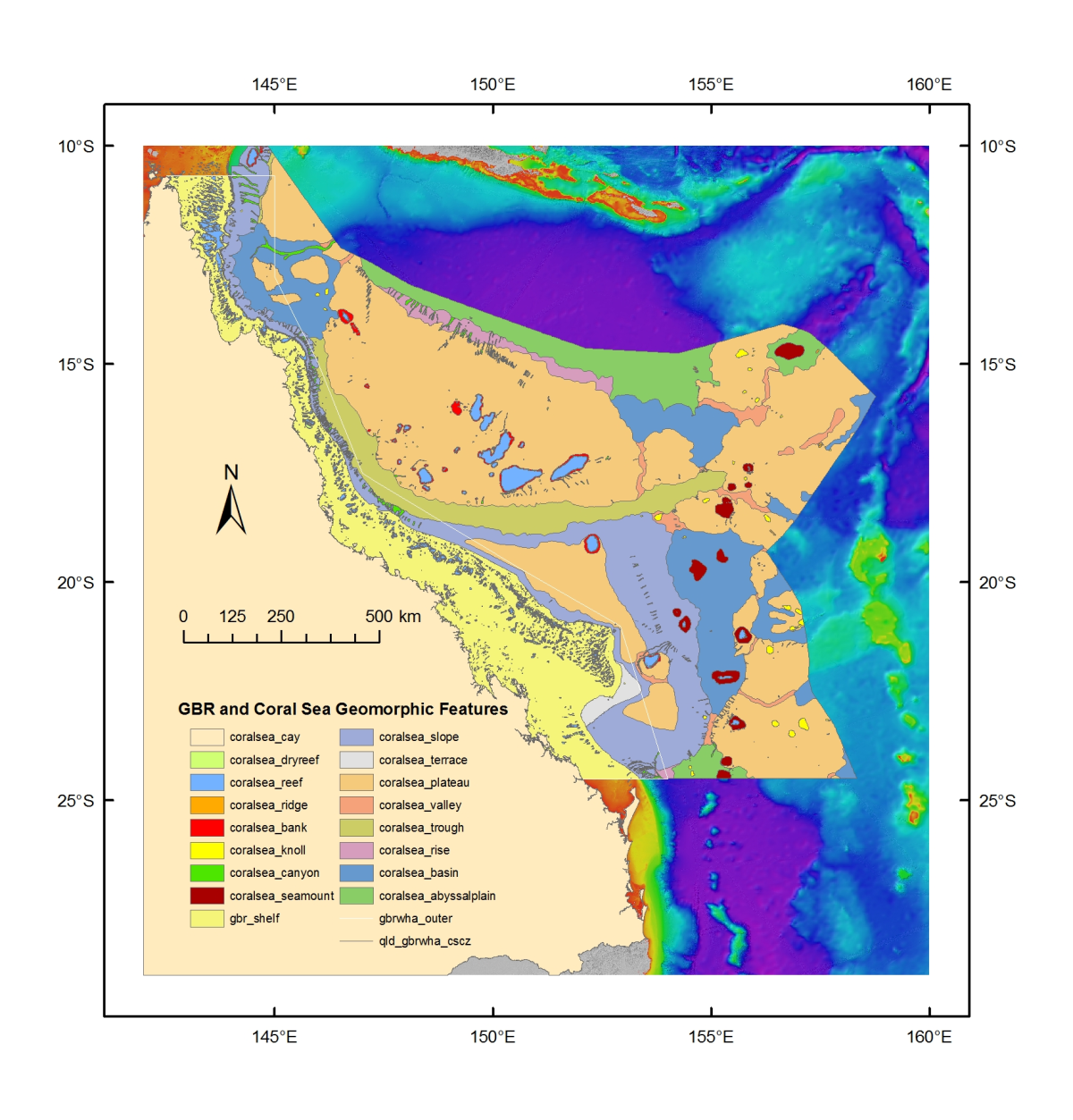
This phase of Project 3DGBR involved manual digitising of geomorphic map boundaries for the key seafloor features identified in the gbr100 grid, particularly for the inter-reefal area on the GBR shelf and in the Coral Sea Conservation Zone (CSCZ). See map for CSCZ boundary at: https://www.environment.gov.au/topics/marine/marine-reserves/coral-sea/conservation-zone Methods: GIS spatial analysis of the gbr100 grid was conducted in order to derive a number of useful background datasets for assisting in the digitising process, such as slope, aspect, hillshading, and dense contour lines. The digitising initially focused on the deep-water (>100 m) environment to develop geomorphic maps for the continental slope, Queensland and Townsville Troughs lying within the Great Barrier Reef World Heritage Area (GBRWHA), and for the Queensland Plateau, Coral Sea Basin, Tasman Basin, and Lord Howe Rise area lying within the adjoining Coral Sea Conservation Zone (CSCZ). The project lastly focuses on the shallow-water (<100 m) environment to develop geomorphic maps for the GBR shelf to complement the shallow reef feature maps provided by GBRMPA. These shallow-water geomorphic features will be added to the project as they come available. Format: This dataset consists of 21 shapefiles and a GeoTiff raster file containing hillshading. Each of the shapefiles is described below. Group Layer 1. Boundaries: gbrwha_outer.shp This Great Barrier Reef World Heritage Area (GBRWHA) layer was initially provided by GBRMPA using a GDA94 datum. The shapefile was reprojected to the WGS84 datum, and then the western coastline boundaries deleted to derive a line shapefile showing only the outer boundary of the GBRWHA where it extends away from the mainland. qld_gbrwha_cscz.shp This line shapefile combines both the GBRWHA and Coral Sea Conservation Zone (CSCZ) areas, with a western boundary limit at the Queensland mainland coastline. This area was used to clip all geomorphic features created in this project. Group Layer 2. GBRMPA features: gbr_dryreef.shp The GBR shelf dryreefs shapefile was initially provided by GBRMPA for this project using a GD94 datum. The shapefile was reprojected to the WGS84 datum and not modified in any other way. It is provided here only for completeness but and products using this shapefile should also acknowledge GBRMPA (see under licensing). gbr_features.shp The GBR shelf features were initially provided by GBRMPA for this project using a GDA94 datum. The shapefile was reprojected to the WGS84 datum, and then the Ashmore Reef polygon deleted due to a grossly incorrect position. The shapefile comprises Cay, Island, Mainland, Reef, Rock and Sand features. Users may contact GBRMPA to obtain details for the creation of these features. Any products using this shapefile should also acknowledge GBRMPA (see under licensing). Group Layer 3. Finer-scale features: coralsea_cay.shp Cay is a sand island elevated above Australian Height Datum (AHD), and located on offshore coral reefs and seamounts. Cays were mapped initially using a shapefile provided by Geoscience Australia for this project, and then their boundaries checked or remapped using Landsat imagery as background source data to help delineate the white sand areas against the surrounding ocean. coralsea_dryreef.shp Dryreef is rock/coral lying at or near the sea surface that may constitute a hazard to surface navigation. Dryreefs were mapped initially using a shapefile provided by Geoscience Australia for this project, which identified those reef areas lying above approximately Lowest Astronomic Tide (LAT). Landsat imagery was used as background source data to check or remap their boundaries. coralsea_reef.shp Reef is rock/coral lying at or near the sea surface that may constitute a hazard to surface navigation. For this project, the boundaries of reef areas were mapped to show the outer-most extent of each coral reef that could be observed in Landsat imagery, thus identifying the greatest area of each reef observed in the Coral Sea. This methodology is consistent with the methodology used to map the outer-most extents of reefs on the GBR shelf conducted by GBRMPA. coralsea_ridge.shp Ridge is a long, narrow elevation with steep sides. In this project, ridges were mapped as widely-scattered and uncommon, finer-scale features identified in the gbr100 grid. These elongate ridges are distinct from the smaller knolls or hills which have a more rounded shape. They are usually found on the plateaus of the Lord Howe Rise. coralsea_bank.shp Bank is an elevation over which the depth of water is relatively shallow but normally sufficient for safe surface navigation. In this project, banks were mapped as the base or pedestal boundaries of the coral reefs found in the Coral Sea. For example, the coral atolls and reefs on the Queensland Plateau are considered banks and their bases digitised where they emerge from the surrounding flat seafloor. coralsea_knoll.shp Knoll is a relatively small isolated elevation of a rounded shape. This shapefile also includes Abyssal hill, a low (100 – 500 m) elevation on the deep seafloor. For this project, knolls and abyssal hills were mapped using background datasets that showed relatively steep changes in elevation contours and variations in slope gradients. Knolls are numerous throughout the Coral Sea area and are greatly underestimated. coralsea_canyon.shp Canyon is a relatively narrow, deep depression with steep sides, the bottom of which generally has a continuous slope, developed characteristically on continental slopes. Canyons were mapped by closely following the narrow sides of canyon axes, digitising from the foot of the canyon where they merge with the surrounding basin floor, and up to the canyon head and into any connecting side gullies. This project identified numerous canyons on any slope gradient >1° and are also greatly underestimated across the area. coralsea_seamount.shp Seamount is a large isolated elevation >1000 m in relief above the seafloor, characteristically of conical form. This shapefile also includes Guyot, a seamount having a comparatively smooth flat top. Seamounts and guyots were mapped mostly within the Tasmantid Seamount Chain with elevations >1000 m. This project identified several large knolls and hills close to 1000 m in height within this chain that may also be seamounts but currently lack detailed bathymetry data. Group Layer 4. Broader-scale features: gbr_shelf.shp Shelf is a zone adjacent to a continent (or around an island) extending from the low water line to a depth at which there is usually a marked increase of slope towards oceanic depths. The eastern boundary of the Queensland continental shelf was mapped by closely following the change in gradient along the shelf edge. The shelf break in the north was at approximately 80 m and became deeper at about 110 m towards the south. The western boundary was clipped at the Queensland mainland coastline. coralsea_slope.shp Slope lies seaward from the shelf edge to the upper edge of a continental rise or the point where there is a general reduction in slope. The continental slope was mapped lying adjacent to the shelf and extending into the adjacent deep basins and troughs. The shelf feature was used to erase the western boundary of the slope and the various basins and troughs erased the eastern slope border. The slope has extensive canyons incising its surface. coralsea_terrace.shp Terrace is a relatively flat horizontal or gently inclined surface, sometimes long and narrow, which is bounded by a steeper ascending slope on one side and by a steeper descending slope on the opposite side. In this project, one broad-scale terrace feature was mapped lying on the slope between the Swains Reefs and Capricorn-Bunker Group of reefs, and near the Capricorn Trough. coralsea_plateau.shp Plateau is a flat or nearly flat area of considerable extent, dropping off abruptly on one or more sides. Extensive areas of plateaus were mapped across the Coral Sea with the largest being the Queensland Plateau. Lord Howe Rise consists of a series of plateaus separated by broad-scale valleys linking adjacent basins and troughs. Plateau boundaries were mapped around their bases where the gradient first becomes steeper. The exceptions are the Marion and Saumarez Plateaus on the Queensland continental slope, where the boundaries were mapped as the slope gradient becomes flat or nearly flat. coralsea_valley.shp Valley is a relatively shallow, wide depression, the bottom of which usually has a continuous gradient. This term is generally not used for features that have canyon-like characteristics for a significant portion of their extent. The shapefile includes Hole, a local depression, often steep sided, of the seafloor. Valleys and holes were mapped as long shallow depressions that often separated the numerous plateaus. These features link the basins and troughs that surround these plateaus, and in some cases can be incised with finer-scale canyons. coralsea_trough.shp Trough is a long depression of the seafloor characteristically flat bottomed and steep sided and normally shallower than a trench. In this project, two trough features were mapped that are essentially long basins. The larger feature is a combined Queensland and Townsville Trough lying between the continental slope and the Queensland Plateau. The smaller feature is the Bligh Trough separating the northern slope and Eastern Plateau. Both trough features feed into the Osprey Embayment and huge Bligh Canyon. coralsea_rise.shp Rise is a gentle slope rising from the oceanic depths towards the foot of a continental slope. For this project, an elongate rise is mapped between the Queensland Plateau and the adjacent Coral Sea Basin. The Queensland Plateau is remnant continental crust from the Gondwana breakup and so its seaward edge provides a geomorphic extension of the Australian margin, albeit at a much deeper depth than the present mainland margin. The rise was mapped where the gradient angle of the Queensland Plateau seaward edge first becomes less steep and finishes at the Coral Sea Basin abyssal plain. Another rise feature was mapped between the southern continental slope and the Tasman Basin abyssal plain. coralsea_basin.shp Basin is a depression, characteristically in the deep seafloor, more or less equidimensional in plan and of variable extent. Basins were mapped where their boundaries changed from generally flat to more steep gradients. Plateau or slope features were used to erase and limit the boundaries of the basin features. In the north lies the large Osprey Embayment which has smaller plateaus lying within its area. The Cato Trough is a large basin separating the southern continental slope and plateaus of the Lord Howe Rise area. On the Lord Howe Rise are shallow basins that surround the series of plateaus that lie on the Lord Howe Rise. coralsea_abyssalplain.shp Abyssal plain is an extensive, flat, gently sloping or nearly level region at abyssal depths. Three abyssal plains were mapped where their gradients became generally flat and at depths greater than about 4000 m. In the north are the abyssal plains of the Coral Sea Basin and Louisiade Basin, the latter being a failed arm of a rift triple junction. In the south, lies the abyssal plain of the Tasman Basin. Group Layer 5. Background image: gbr100_geo3.tif This hillshade geotif image was derived from the gbr100 grid using Fledermaus 3D visualization software with a depth colour scheme configured to highlight the physiographic relief of the shallow shelf and the deeper seabed features. It is provided here to give geomorphic context to the seabed areas lying outside of the GBRWHA and CSCZ. Funding: Queensland Government Smart Futures Fellowship Reef and Rainforest Research Centre James Cook University References: Heap, A.D., Harris, P.T., 2008. Geomorphology of the Australian margin and adjacent seafloor. Australian Journal of Earth Sciences 55(4), 555-585. doi: 10.1080/08120090801888669 IHO, 2008. Standardization of Undersea Feature Names: Guidelines, Proposal Form, Terminology. Bathymetric Publication No.6, 4th Edition, International Hydrographic Bureau/Intergovernmental Oceanographic Commission, Monaco, pp. 32. Change log: 2023-01-10 - Updated the dataset download link from the original JCU link that is broken (http://ftt.jcu.edu.au/deepreef/3dgbr/geo/3dgbr_geomorph.zip) to a cached version hosted by the eAtlas.

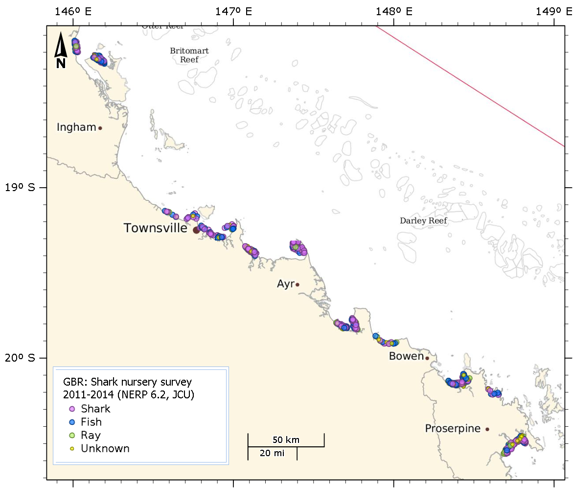
This dataset contains the catch data from seasonal gillnet and longline surveys of shark nursery areas in the Central Section of the Great Barrier Reef Marine Park (2011-2014). Methods: Sampling occurred seasonally in nine bays along ~ 400 km of the tropical north Queensland coastline: Rockingham, Halifax, Cleveland, Bowling Green, Upstart, Abbott, Edgecumbe, Woodwark/Double and Repulse Bays. Of these nine bays, five were sampled regularly, the others (in italics) were sampled only once as part of a broader survey. Sampling sites were dominated by silty substrates, and mudflat and/or mangrove-lined foreshores. Between October 2011 and November 2013 eight rounds of fisheries-independent surveys were undertaken to collect data on the shark community across the study region. Within each bay sampling occurred randomly within sixteen 0.9 km wide strips running perpendicular to the shore. Two groups of eight strips were placed within each bay to spread the sampling across different habitat types and management zones (i.e. gill-net fishing allowed and gill-net fishing prohibited) where possible. During each round, each bay was sampled over four days allowing for two days of sampling in each group of strips. The bays vary in size and so the relative proportion of area sampled varied between bays. Two methods were used to sample across a broad range of shark sizes. During a total of 183 days of sampling, 453 longline shots and 343 gill-net shots were deployed totaling 370 and 310 h, respectively. Bottom-set gill-nets, comprised of 11-cm-stretched mesh, were deployed for ~ 1 h and checked every 15 min to facilitate tagging and release. In accordance with the Great Barrier Reef Marine Park Authority’s Dugong Protection Areas, multiple panels of net were joined to create a total net length of either 200 m or 400 m. In addition, some 100-m gill-nets were used during the Jan/Feb round in 2012. Bottom-set longlines were comprised of 800 m of 6-mm nylon mainline with an anchor and float at both ends. Gangions were attached to the mainline ~ 8–10 m apart; and were comprised of 1 m of 4-mm nylon cord, 1 m of 1.5-mm wire leader, and a baited 14/0 Mustad tuna circle hook. A variety of fresh and frozen baits were used including butterfly bream (Nemipterus sp.), squid (Loligo sp.), blue threadfin (Eleutheronema tetradactylum) and mullet (Mugil cephalus). Up to two longlines were deployed simultaneously for 40–90 min sets. Environmental data (water temperature, salinity, depth, turbidity and oxygen saturation) were recorded for all sets. Captured sharks were identified to species level, tagged on the first dorsal fin (Rototag or Superflex tag; Dalton, Oxfordshire, UK), measured, sexed, assessed for clasper calcification, examined for umbilical scar condition, and released at their capture site. Stretch total length was determined according to Compagno (1984). Small sharks (? 1 m) were placed ventral side down on a measuring board and measured to the nearest mm with the upper lobe of the caudal fin depressed in line with the body axis. Larger sharks were secured beside the boat and measured to the nearest cm using a measuring tape. Additional measurements of fork length and pre-caudal length were recorded. Format: CSV File, 4432 rows (~1MB), Shapefiles (4409 Points) Each line of data represents the catch of an individual shark, ray, fish, etc. Multiple lines exist per shot if more than one animal was caught. The shapefile was created by the eAtlas for visualisation purposes. It retains most of the information in the CSV as a point shapefile. The point shapefile was created from the CSV using the Start_Lat and Start_Long as the coordinate for points. If rows which did not have a valid Start_Lat or Start_Long (29 rows) then the End_Lat and End_Long were used instead (6 rows). If neither of these were available then the row was ignored. This removed 23 rows. Attributes Lat and Long were added to contain the coordinates used in the shapefile, leaving the original start and end coordinates untouched. Data Dictionary: Note: The attribute names in rounded brackets () correspond to the name in the shapefile version of the data. These names were adjusted to fit within the 10 character limit of shapefile attributes. - Shot_Code: Unique identifier for each gear shot. - Bay_Code: Bay identifier (AB – Abbott Bay; BG – Bowling Green Bay; CB – Cleveland Bay; ED – Edgcombe Bay; HB – Halifax Bay; RE – Repulse Bay; RO – Rockingham Bay; UP – Upstart Bay; WD – Woodwark/Double Bay) - Round: Round identifier. A combination of the year and a sequential letter unique to the round in that year. - Trip_Start_Date (Trip_Date): sampling date - Fishing_Start (Fish_Start): start time of set (24 hour time) - NERP_Grid: code of the sampling strip used (randomly selected) - Gear_Type: type of gear used (Long-Line or type of gill-net [mesh sizes]) - Number_Hooks (Num_Hooks): If long-line number of hooks. If gill-net then blank. - Gear Length (Gear_Len): length of gear deployed - Mesh size (Mesh_Size): gill-net mesh size (in inches stretched mesh), if long-line then blank - Soak_Hours: time gear was fishing (in hours) - Net_Fishing (Net_Fishin): whether the set was in an area open or closed to net fishing - Lunar Stage (Lunar_Stge): lunar stage on day of sampling (derived from date of set) - Season: season of year (derived from date of set) - Start_Lat: latitude at start of deployment (decimal degrees) (WSG84) - Start_Long: longitude at start of deployment (decimal degrees) (WSG84) - End_Lat: latitude at end of deployment (decimal degrees) (WSG84) - End_Long: longitude at end of deployment (decimal degrees) (WSG84) - Depth: depth of deployment (metres) - Temp: water temperature at deployment (degrees centigrade) - Salinity: salinity at deployment (unitless) - DO: dissolved oxygen level (mgO2) - Secchi_Depth (Secchi_Dep): turbidity as measured by the secchi depth (metres, blank if unmeasured or if secchi disk visible on bottom) - Species_ID: three letter species code of individual (full species name is in Name field) - Species_ID_ElasmosOnly (Sp_ID_Elas): three letter code if an elasmobranch, non-elasmobranchs denoted by dash. - Functional Group (Func_Group): broad taxonomic group of individual (shark, ray, fish) - Maturity stage 3 levels (Mat_stge_3): three stage index of maturity of individual (YOY – young of the year; IM – immature; MAT – mature; UNK – unknown) - Maturity stage 2 levels (Mat_stge_2): two stage index of maturity of individual (IM – immature; MAT – mature; UNK – unknown) - Tag_ID: tag number if individual tagged and released. Tag numbers starting with U designated individuals not fitted with tags (code represents location biological data) - TL: stretched total length of individual (millimetres) - Sex: sex of individual (M – male; F- female; U – unknown) - Fate_ID: fate of the individual (RT – released tagged; RELA – released alive; DD – dead at capture and discarded; RES – retained as a research sample) - Name: species name of individual - Family: family name of individual - Trip_ID: unique identifier for trip Data Location: This dataset is filed in the eAtlas enduring data repository at: data\NERP-TE\6.2_Juvenile-sharks

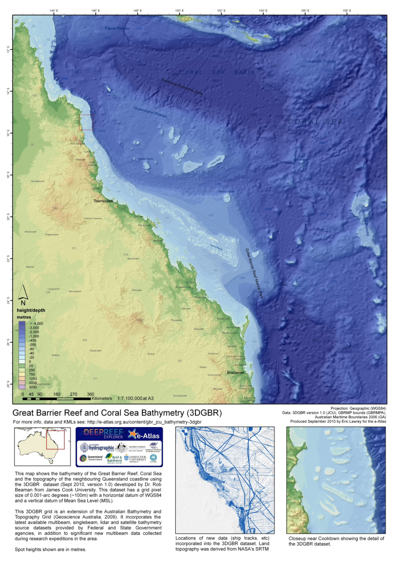
The gbr100 dataset is a high-resolution bathymetry and Digital Elevation Model (DEM) covering the Great Barrier Reef, Coral Sea and neighbouring Queensland coastline. This DEM has a grid pixel size of 0.001-arc degrees (~100m) with a horizontal datum of WGS84 and a vertical datum of Mean Sea Level (MSL). For the latest version of this dataset download the data from http://deepreef.org/bathymetry/65-3dgbr-bathy.html This dataset was developed as part of the 3DGBR project. This grid utilises the latest available multibeam, singlebeam, lidar and satellite bathymetry source datasets provided by Federal and State Government agencies, in addition to significant new multibeam data collected during research expeditions in the area. The large increase in source bathymetry data added much detail to improving the resolution of the current Australian Bathymetry and Topography Grid (Whiteway, 2009). The gbr100 grid provides new insights into the detailed geomorphic shape and spatial relationships between adjacent seabed features. The accompanying report contains an explanation of the various source datasets used in the development of the new grid, and how the data were treated in order to convert to a similar file format with common horizontal (WGS84) and vertical (mean sea level) datums. Descriptive statistics are presented to show the relative proportion of source data used in the new grid. The report continues with a detailed explanation of the pre-processing and gridding process methodology used to develop the grid. A description is also provided for additional spatial analysis on the new grid in order to derive associated grids and layers. The results section provides a short overview of the improvement of the new grid over the current Australian Bathymetry and Topography Grid (Whiteway, 2009). The report then presents the results of the new grid, called gbr100, and the associated derived map outputs as a series of figures. A table of metadata for the current source data accompanies this report as Appendix 1. The report is available at: http://www.deepreef.org/publications/reports/67-3dgbr-final.html Data details and format: gbr100 bathymetry grid: Height/Depth in metres (MSL) Formats: 19000x18000 pixel grid (32 bit float) in ESRI raster grid file, GMT/netCDF grid file, Fledermaus sd file, 100m contour ESRI shapefile, GeoTiff grid file. Total Vertical Uncertainty: Total Vertical Uncertainty (TVU) in the bathymetry estimated from uncertainty classification of each source dataset. Formats: 19000x18000 pixel grid (32 bit float) in ESRI raster, GeoTiff. Hillshading: Hillshading for full gbr100 and also ocean areas only. Derived from the gbr100 grid. Format: 19000x18000 pixel grid (8 bit) in GeoTiff. Funding history: This dataset was initially developed as part of project 2.5i.1 from the MTSRF program (2010). Subsequent versions of the dataset were developed from other funding sources. Version history: - July 2010 - Version 1 Initial release of the DEM. - Dec 2014 - Version 3 This version incorporates dozens of new bathymetric surveys including many new navy LADS surveys and some satellite derived bathy to fill in some gaps left by LADS. - Jan 2016 - Version 4 This version incorporates estimates of bathymetry from satellite imagery in shallow clear waters. - Nov 2020 - Version 6 This revised 3D depth model (V6 – 10 Nov 2020) is a significant improvement on the previous 2017 version, with all offshore reefs mapped with either airborne lidar bathymetry surveys or satellite derived bathymetry. All the available processed multibeam data are now included. Crowdsourced singlebeam bathymetry adds over 50 thousand line km of source data to the inter-reef seafloor. Work will continue to fill the gaps. Data Location: This dataset is filed in the eAtlas enduring data repository at: data\ongoing\GBR_JCU_Beaman_3DGBR-bathymetry-gbr100 Note: Copies of legacy versions 1, 3 and 4 are stored in the eAtlas and available on request. eAtlas Processing: To visualize this dataset on the eAtlas the format of the data was converted from the ESRI ArcInfo grid format into a GeoTiff format. This was done by loading the data in ArcMap then exporting it as a GeoTiff image. Overview images and final compression options were then performed using GDAL tools.